Descriptive Statistics VS Inferential Statistics

• Descriptive - is about describing our collected data using the measures discussed throughout this lesson: measures of center, measures of spread, shape of our distribution, and outliers. We can also use plots of our data to gain a better understanding.

---

• Inferential - is about using our collected data to draw conclusions to a larger population. Performing inferential statistics well requires that we take a sample that accurately represents our population of interest.

A common way to collect data is via a survey. However, surveys may be extremely biased depending on the types of questions that are asked, and the way the questions are asked. This is a topic you should think about when tackling the the first project.

1. Population - our entire group of interest.
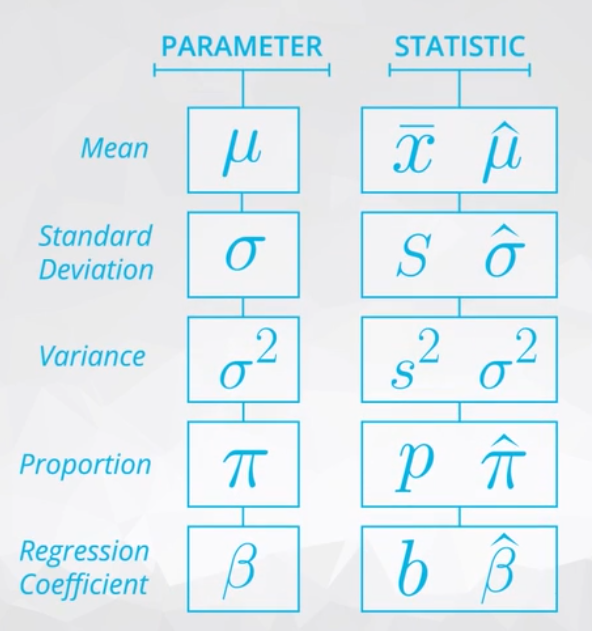
2. Parameter - numeric summary about a population
3. Sample - subset of the population
4. Statistic numeric summary about a sample

QUIZ QUESTION Identify the population, parameter, sample, and statistic for the below scenario:

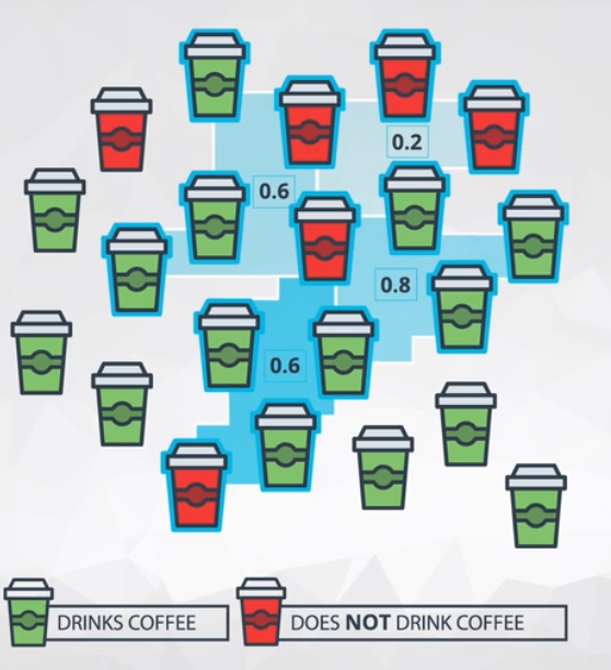
Consider we are interested in the average number of hours slept by all Udacity students (100,000 students). I send an email to all Udacity students, but I only receive 5,000 response emails. The average amount of sleep of those that responded was 6.8 hours of sleep.

Population All Udacity Students Parameter We cannot know for sure Sample 5,000 Udacity students Statistic 6.8 hours of sleep

Statistics and parameters are generally the mean or proportion for a group. Statistics being the value for the sample. Parameters being the value for the population. The population is our entire group of interest, while a sample is the selected subset of the population.

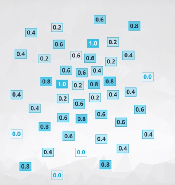
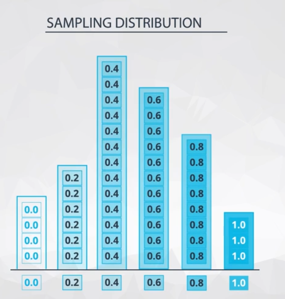
A sampling distribution is the distribution of a statistic.

Sampling Distributions Quiz

Sampling Distributions Solutions

Sampling Distributions Notes

• Sampling Distributions are the distribution of a statistic (any statistic).

• There are two very important mathematical theorems that are related to sampling distributions: The Law of Large Numbers and The Central Limit Theorem.

We have already learned some really valuable ideas about sampling distributions:

First, we have defined sampling distributions as the distribution of a statistic.

This is fundamental - I cannot stress the importance of this idea. We simulated the creation of sampling distributions in the previous ipython notebook for samples of size 5 and size 20, which is something you will do more than once in the upcoming concepts and lessons.

Second, we found out some interesting ideas about sampling distributions that will be iterated later in this lesson as well. We found that for proportions (and also means, as proportions are just the mean of 1 and 0 values), the following characteristics hold.

The sampling distribution is centered on the original parameter value.

The sampling distribution decreases its variance depending on the sample size used. Specifically, the variance of the sampling distribution is equal to the variance of the original data divided by the sample size used. This is always true for the variance of a sample mean!

In notation, we say if we have a random variable, , with variance of , then the distribution of (the sampling distribution of the sample mean) has a variance of

Notation

Notation Quiz

Law of Large Numbers

• The Law of Large Numbers states that as a sample size increases, the sample mean will get closer to the population mean. In general, if our statistic is a “good” estimate of a parameter, it will approach our parameter with larger sample sizes.

Central Limit Theorem

• Central Limit Theorem states that with large enough sample sizes our sample mean will follow a normal distribution, but it turns out this is true for more than just the sample mean.

Central Limit Theorem Part 1

The sample size above wasn’t large enough for CLT to take effect.

Central Limit Theorem Part 2

The sample size of 100 is large enough for CLT to take effect.

CLT Notes

• Mean and Proportion are normally distributed with large enough sample sizes. But, when is it large enough?

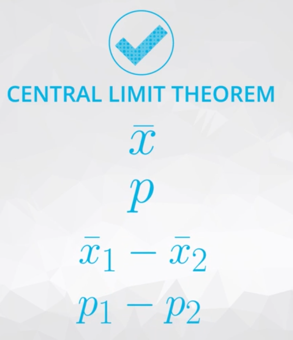
• CLT applies to: Mean, Proportion, difference of mean, difference of proportion

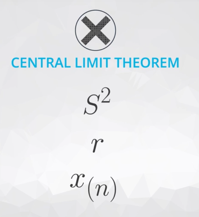
• CLT does not apply to: sampling distribution of the variance, correlation coefficient, sampling distribution for maximum value of the dataset

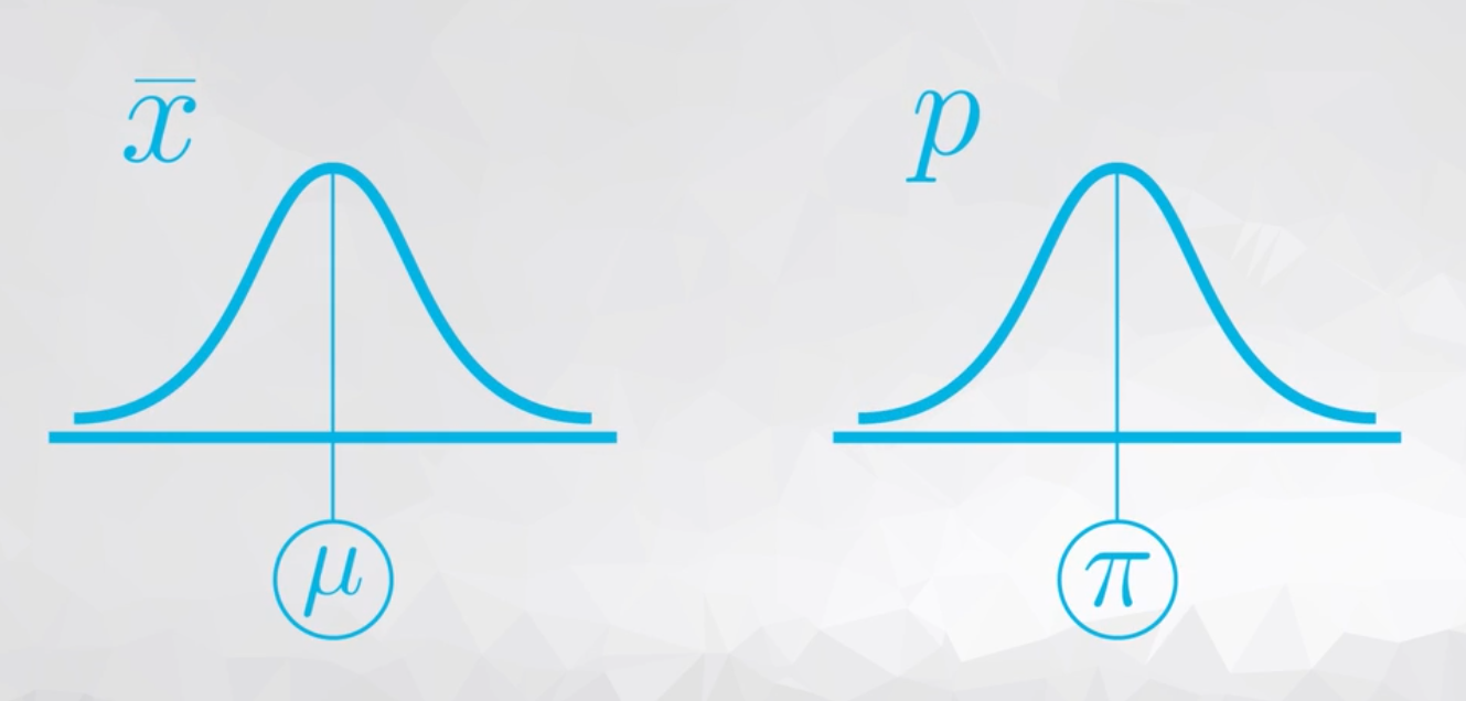
You saw how the Central Limit Theorem worked for the sample mean in the earlier concept. The Central Limit Theorem states that with a large enough sample size the sampling distribution of the mean will be normally distributed.

The Central Limit Theorem actually applies for these well known statistics:

1. Sample means ()

2. Sample proportions ()

3. Difference in sample means ()

4. Difference in sample proportions ()

And it applies for additional statistics, but it doesn’t apply for all statistics.

Central Limit Theorem Part 3

• This distribution is right skewed, not normally distributed.

Bootstrapping

• Bootstrapping is a technique where we sample from a group with replacement.

• We can use bootstrapping to simulate the creation of sampling distribution, which you did many times in this lesson.

• By bootstrapping and then calculating repeated values of our statistics, we can gain an understanding of the sampling distribution of our statistics.

Bootstrap Sampling

Top